Natalie Lamb and the RNA-seq Analysis for Beginners

This blog post has been produced after a training course at the University of Sheffield "RNA-seq Analysis for Beginners Training course". It will cover:

• Performing quality assessment on our fastq files
• Aligning fastq files to the reference genome
• Visualising the reads in IGV
• Counting against a set of reference transcripts

This essentially means what to do with raw RNA data (fastq) using the steps: Quality Control (fastqc) - Alignment (hisat2) - Counting (htseq) - Differential Expression (deseq2) - Pathways using Galaxy.

Upload Data

In Galaxy, an open, web-based platform for data intensive biomedical research, search upload in the "tools" section on the left hand side and select "Upload File". On the right hand side, each data set will be red. When uploaded, this will turn green.


Quality Control

Click "View" (the small eye icon next to the green data set) to see the fastq file. Fastq files are text files that describe the sequence. Each "read" is described by four lines: the sequence ID, the sequenced read, a blank (+) and the quality score (a long series of jibberish).

The quality (Q) scores are representations of how confident we are that a particular base has been called correctly (the base call probability). Each symbol has a meaning using the ASCII code. Letters that are further along the alphabet indicate higher confidence. The Q score is worked out using the formula Q=−10log10p using software. Some examples of Q scores:

• Q = 30, p=0.001
• Q = 20, p=0.01
• Q = 10, p=0.1

Tools such as "FastQC Report" will read this score and translate it into a format that makes more sense, such as the below image. Green=passes, red=fails. Search "FastQC Report Quality Reports" in the "Tools" search bar. Under the heading "Short read data from your current history" select the desired file using the icon on the right under this heading. Click "Execute". This will produce images such as the below for the data set you selected.

As in the above image, the quality score will often decrease over time as reagents age, meaning that often the last 10 base pairs are cut off.

Using MultiQC will allow you to compare multiple data sets at the same time, rather than FastQC Report which only allows you to see one data set at a time. In "Tools" search and select "MultiQC". Under "Which tool was used generate logs?" select "FastQC". Then select all the files with the name "Raw Data" then click "Execute".

Alignment

Alignment is for determining where each of the reads come from. This is because both the genome you are trying to work with and the genome which is for reference use (so has already been decoded, so to speak) have both been broken down into fragments to make it quicker to find matches.

To do it, search "HISAT2" in "Tools". In the data set I was using, under the heading "Select a reference genome" I had to select "S. cerevisiae Apr. 2011 (SaccCer_Apr2011/sacCer3) (sacCer3)" but this depends on the species being used. Under the heading "FASTA/Q file either select a single or multiple files that you want to complete alignment on then click "Execute". It will produce bam files. These files give the location where each read is lined to.

Under the heading "QNAME", there are the names (SN) of the sequences (chromosomes) used in alignment (e.g. chrI is chromosome number 1) and their length (LN).

The below is what all the heading mean:

Under the "FLAG" heading there will be a number. This can be searched for using this website to find out what that specific number means.

Flagstat (search for it in "Tools") will calculate the flag for each read in the bam file and tabulate the results. Don't forget to select multiple files if you are working with more than one data set. In the below example, the aligned percentage is 99.95%.

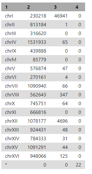
Idxstats (search for it in "Tools") will report the number of reads mapping to each reference sequence (i.e. chromosome).

To visualise the alignments, open Integrative Genomics Viewer (IGV), a different software from Galazya which is a "high-performance visualization tool for interactive exploration of large, integrated genomic datasets" (IGV, 2019). It is ofetn used as a first pass at visualising NGS data (Next generation sequencing is a new method for sequencing genomes at high speed and at low cost).

In Galaxy, download the bam files you created in Galaxy by clicking on the data set and then the save icon on the right-hand panel. Download both the Download data set and Download index buttons.

In IGC, click the drop down in the top left and select the organism who you are working with. The bit at the bottom shows the genes present in the reference organism you have selected (i.e. the reference genome that has already been decoded). Click "File" then "Upload" and select all your bam files.

 In the box next to the organism, you can select a specific chromosome to look at it. In the above example, I am looking at Chromosome 1. You can also use the mouse to drag left and right.


Counting

After alignment, the next step is to count the number of tomes a specific gene has been sequenced. Longer genes will get more reads because there is more of them (the entire gene doesn't have to match, just bits of them).

In Galaxy, search and select "UCSC Main table browser" in "Tools". I used the following settings:

• Set clade to Other
• Set genome to S. cerevisiae
• assembly Apr. 2011
• group Genes and Gene Prediction
• track SGD Genes
• region genome
• output format GTF - gene transfer format (limited) and send output to Galaxy

Click "Get Output" and then "Send Query to Galaxy"

Then search and select "htseq-count" in "Tools". Select all the bam files and make sure that "GFF File" is on the correct organism. Then click "Execute".


Differential Expression 

The term differential expression was first used to refer to the process of finding statistically significant genes from a microarray gene expression study. RNAseq has now replaced microrrays, although they can still be used. Basically it means that you've counted the genes but now you need stats to prove you've the genes you've counted are all differentially expressed.

For example in the below image, A has a different average differential experession than B but there is variability/range.

In Galaxy, search and select "DESeq2" in "Tools. I used the following parameters:

• 1. Factor level: Input Batch
• Count files: batch1-htseq, batch2-htseq
• 2. Factor level: Input Chem
• Select columns containing control: chem1-htseq, chem2-htseq
• For Output normalized counts table select "Yes"

Click "Execute"

Search and select "Filter" in tools. I used the following conditions:

• Filter: DESeq2 results file
• With following condition: c7 < 0.05 and (c3 > 1.0 or c3 < -1.0)
• Number of header lines to skip: 1

Click "Execute". This will extract the significant differentially expressed genes, such as those below.

Search "Column Join" using "Tools" and select all the htseq files. Click on this on the right hand side and click save to download this file.

Degust is a web tool that can analyse the counts files produced in the step above, to test for differential gene expression. It offers and interactive view of the differential expression results. Upload the file created by clicking "Upload your counts file". I used the following parameters:

• For "Name" type “DGE in SaCer3” (or whatever you want to call the analysis)
• For "Info Columns" select “#KEY”
• For "Analyze Server Side" leave box checked.
• Click "Add Condition" and name the different conditions e.g. "Batch" and "Chem"
• Save the settings and then click "View The Results"

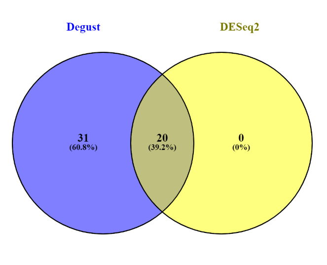
The website Venny computes overlaps in gene lists so this could wither be between experiment conditions (e..g. batch vs chem) or through genes identified using different methods (e.g. DESeq2 and Degust). Open both the DESeq2 and Degust results files in Excel. Copy the names (e.g. YAR002C-A) of the DESeq2 data set which have a p-value less than 0.05 into the top-left box on the Venny website (List 1). Do the same for the names of the Degust data set, again with a p-value less than 0.05 into List 2. 

And there we have it, how to do some basic RNA-seq analysis!

References

1. Dunning, M (2019), Hands-on RNA-seq Analysis in Galaxy, based on the RNA-Seq Workshop by Melbourne Bioinformatics written by Mahtab Mirmomeni, Andrew Lonie, Jessica Chung Original, modified by David Powell (Monash Bioinformatics Platform), further modified by Mark Dunning of Sheffield Bioinformatics Core.
2. Nookaew I, Papini M, Pornputtpong N, Scalcinati G, Fagerberg L, Uhlén M, Nielsen J (2010), A comprehensive comparison of RNA-Seq-based transcriptome analysis from reads to differential gene expression and cross-comparison with microarrays: a case study in Saccharomyces cerevisiae. Nucleic Acids Res 2012, 40 (20):10084 – 10097. doi:10.1093/nar/gks804. 
3. Guirguis A, Slape C, Failla L, Saw J, Tremblay C, Powell D, Rossello F, Wei A, Strasser A, Curtis D (2016), PUMA promotes apoptosis of hematopoietic progenitors driving leukemic progression in a mouse model of myelodysplasia. Cell Death Differ. 23(6).